Understanding Control Systems and use in Plant Control (MFCNTRL & LBYMF3I)

TARGET AUDIENCE: Self, Students, Academics, Industry Professionals, Employers, and Tech Enthusiasts

Note:

OVERVIEW: One of the main things that I was able to absorb throughout my stay in MEM is the concept of closed-loop control systems and the use of propotional-integral-derivative (PID) controllers. Below is the competencies and exploration that I made to understand the theoretical and practical ‘standings going into real-world uses for this type of automation.

LECTURE:

The principles that govern open- and closed-loop control to PID regulation will consider differential equations on the time domain. The better the design to minimize the error in the second for the output to reach the desired input that is where you can confidently say that you have a functioning control system. Below are the concepts that we had to learn to make this work:

Open-Loop Systems:

An open-loop control system acts solely on the input and does not use feedback to correct its output.

General Form:
\(C(s) = G(s)R(s)\)

Where:

• \(R(s)\) = input (reference signal)
• \(C(s)\) = output (controlled variable)
• \(G(s)\) = system or plant transfer function

Key Insight: Open-loop systems are simple but cannot adapt to disturbances or system changes.

Closed-Loop Systems with Feedback:

In closed-loop systems, the output is compared to the input, and the error is fed back to reduce deviations.

General Form:
\(C(s) = \frac{G(s)}{1 + G(s)H(s)} R(s)\)

Where:

• \(H(s)\) = feedback transfer function

Key Insight: Closed-loop systems are more complex but provide stability, accuracy, and disturbance rejection.

Standard Input Signals

Control system performance is tested against standard signals:

1. Unit Pulse (Impulse):
   \(\delta(t) = \frac{du(t)}{dt}\)

2. Unit Step:
   \(u(t) = \begin{cases} 0, & t < 0 \\ 1, & t \geq 0 \end{cases}\)

3. Unit Ramp:
   \(r(t) = t \cdot u(t)\)

Key Insight:

• Step response → measures system stability.
• Ramp response → measures system tracking.
• Impulse response → reveals natural dynamics.

Partial Fraction Expansion & Decomposition

When analyzing transfer functions, rational expressions are often decomposed into simpler terms using partial fractions.

Example:
\(\frac{Y(s)}{U(s)} = \frac{1}{(s+2)(s+3)}\)

Decomposition:
\(\frac{1}{(s+2)(s+3)} = \frac{A}{s+2} + \frac{B}{s+3}\)

Where constants \(A\) and \(B\) are found algebraically.

Key Insight: Partial fraction expansion simplifies inverse Laplace transforms, making it easier to compute time-domain responses.

Matrix Multiplication and Determinants

Control systems often use state-space representation. This is commonly seen in circuit systems when doing KVL where we had to know this and also determine the transfer function of an RLC circuit. To be simplify work, you need to know matrix operations.

\[\dot{x}(t) = Ax(t) + Bu(t)\] \[y(t) = Cx(t) + Du(t)\]

Where:

• \(A\) = system matrix
• \(B\) = input matrix
• \(C\) = output matrix
• \(D\) = feedthrough matrix

To find system properties (e.g., stability), we calculate determinants:

\[\text{det}(AB) = \text{det}(A) \cdot \text{det}(B)\]

Key Insight: This property is used in solving systems of equations and in finding eigenvalues(solutions of the equivalent ODE linear alg!) for stability analysis.

Systems of Equations & Higher-Order Transfer Functions

For increasing system orders, differential equations are solved using Laplace and algebraic manipulation:

Example (2nd-order system):
\(\frac{d^2 y(t)}{dt^2} + a_1 \frac{dy(t)}{dt} + a_0 y(t) = b_0 u(t)\)

Laplace domain:
\(G(s) = \frac{Y(s)}{U(s)} = \frac{b_0}{s^2 + a_1 s + a_0}\)

Key Insight: Higher-order systems require systematic methods (state-space, Laplace, matrix inversion) to derive transfer functions.

PID Control – Terms & Time-Response Effects

PID Controller regulates a system by combining proportional, integral, and derivative actions:

\[u(t) = K_p e(t) + K_i \int e(t) dt + K_d \frac{de(t)}{dt}\]

Where \(e(t) = r(t) - y(t)\) is the error signal.

Term Effects:

• Proportional (\(K_p\)):
  Increases responsiveness, reduces steady-state error but may cause overshoot.

• Integral (\(K_i\)):
  Eliminates steady-state error by accumulating past errors.

• Derivative (\(K_d\)):
  Predicts future error, improves stability, reduces overshoot.

Key Insight: Tuning PID gains shapes the time response (rise time, overshoot, settling time, steady-state error).

Below is a consolidattion of my notes that I have for this lecture that I have thankfully digitized.

I have also here the calculations that I have done in attempt to solveour finals exams. There was no feedback on the errors in my calculations but I got a solid 40/50 out of this so pretty confident in my answers :)) I think other exams were done F2F so I was not capture the solutions that I have made

LABORATORY:

In this series of lab projects that I have made for this course, I was able explore the fundamentals of control systems—from deriving and manipulating transfer functions using Laplace transforms in MATLAB, to implementing practical setups with FESTO EduKit and COM3Lab modules. The work focused on understanding system dynamics, stability, and the role of controllers like PID, bridging the gap between theory and industrial application.

🔬 Methodology and Key Work

Lab 1. Transfer Functions & Laplace Analysis

Control systems begin with the modeling of differential equations. I started with modeling dynamic systems using differential equations and converting them into algebraic forms via Laplace transforms.

For a standard LTI (Linear Time-Invariant) system:

\[\frac{d^n y(t)}{dt^n} + a_{n-1}\frac{d^{n-1} y(t)}{dt^{n-1}} + \dots + a_0 y(t) = b_m \frac{d^m u(t)}{dt^m} + \dots + b_0 u(t)\]

Applying the Laplace Transform converts this into an algebraic equation:

\[Y(s)\big(s^n + a_{n-1}s^{n-1} + \dots + a_0 \big) = U(s)(b_m s^m + \dots + b_0)\]

Thus, the Transfer Function is:

\[G(s) = \frac{Y(s)}{U(s)} = \frac{b_m s^m + \dots + b_0}{s^n + a_{n-1}s^{n-1} + \dots + a_0}\]

I was able to do the follow:

• Used tf(num, den) to define transfer functions.
• Applied residue(num, den) for partial fraction expansion.
• Plotted poles and zeros with pzmap(G).

2. Continuous-Time Signals

In MATLAB, various input signals were simulated to uprich still on signal behavior for control systems in both time and frequency domains. Below is the functions that we tackled:

• Unit Step Function:
  \(u(t) = \begin{cases} 0, & t < 0 \\ 1, & t \geq 0 \end{cases}\)

• Impulse Function:
  \(\delta(t) = \frac{du(t)}{dt}\)

• Exponential Input:
  \(x(t) = e^{-at}u(t)\)

• Sinusoidal Input:
  \(x(t) = A \sin(\omega t + \phi)\)

I was able to do the following:

• Generated with step(G), impulse(G), and lsim(G, u, t).
• Verified stability from bounded inputs → bounded outputs (BIBO stability).

---

3. FESTO EduKit: Fluid Dynamics & Flow Control

A practical setup was used to study flow vs. resistance vs. pressure. With the hands-on fluid dynamics to see how pressure, resistance and flow interact. This goes outside the assumption that control systems consider only on the electronics side but can also be applied in physical systems!!

Governing Formula (Bernoulli + Flow Resistance)

\(Q = \frac{\Delta P}{R}\)

Where:

• \(Q\) = volumetric flow rate
• \(\Delta P\) = pressure difference
• \(R\) = flow resistance

Findings: Increasing valve resistance caused higher upstream pressure but reduced flow rate.

• Adjusted valves to vary flow resistance.
• Recorded effects on pressure and flow rate.
• Confirmed inverse relationship between resistance and flow.

4. COM3Lab Open- vs. Closed-Loop Control

We further explored the use of loop control under the use of FESTO’s COM3ab. We were able to control a simple fan in a cooling system that maintend temperature in varying environment conditions.

Open-Loop System

No feedback — output does not affect input.
\(C(s) = G(s)R(s)\)

Closed-Loop System with Feedback

\(C(s) = \frac{G(s)}{1 + G(s)H(s)} R(s)\)

Where:

• \(R(s)\) = reference input
• \(C(s)\) = controlled output
• \(G(s)\) = plant transfer function
• \(H(s)\) = feedback transfer function

PID Control Law

\(u(t) = K_p e(t) + K_i \int e(t) dt + K_d \frac{de(t)}{dt}\)

Where:

• \(\(K_p\)\) = proportional gain
• \(\(K_i\)\) = integral gain
• \(\(K_d\)\) = derivative gain
• \(\(e(t) = r(t) - y(t)\)\) is the error

Experiment:

• Open-loop: Temperature fell rapidly when disturbed by a fan.
• Closed-loop: PID maintained target temperature despite disturbance.
• Verified system linearity via static input-output plots.

Below is a consolidated document of the lab reports that we submitted for viewing.

Final Project

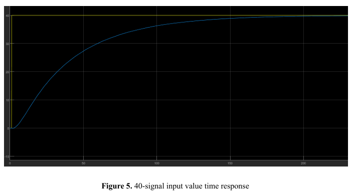
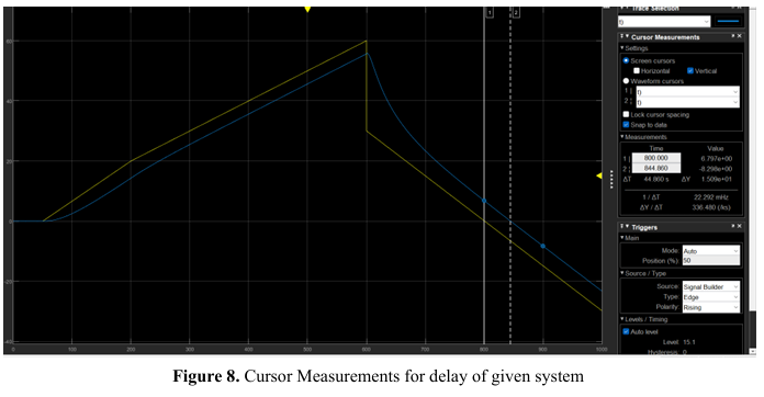
For my final project of learning these concepts, I tasked myself to replicate a study with a known transfer function and model its time reponse via MATLAB. I chose to discusses the modeling and simulation of a Single Input, Single Output (SISO) system for ammonium removal from a sand biofilter in a wastewater treatment plant (WWTP). It emphasizes the use of a Proportional-Integral-Derivative (PID) controller to optimize the removal process, focusing on the initial concentration of ammonium as the input parameter.

The study incorporates a closed-loop Simulink block to derive mathematical equations and visualize system responses. I have change slightly that controller parameters in order to optimize the response compared to the reference study. The results indicate that the tuned PID parameters from this study are smaller than those from a reference study, suggesting potential improvements in the control strategy for ammonium removal efficiency.

Below is a copy of our project report. I must note though that the instructor at the time has expressed incorrect modelling on our end but no feedback to correct it. On my end reflecting on this, I think the issue was that the input signal was immediate which maybe is not desired despite my correct use of the transfer function. I was not able to truly capture the difference of the simulated reponse to the desired reponse for the SISO system that resulted to the confusion on what params should be controlled by the instructor too.

Learnings and Reflection:

The whole experience has thought me the use of Laplace transforms from our calculus days that will simplify analysis of dynamic systems. The use of Poles and zeros as critical indicators of system stability especially when we are dealing with the time-frequency domain. The FESTO experiments were fun, at least for me, that I was able to configure and demonstrate fluid control principles (pressure-flow-resistance) as well as Closed-loop control with PID to ensure stability, accuracy, and disturbance rejection. Lastly, the use of MATLAB software as a tool for bridging equations to simulations, while FESTO/COM3Lab brings theory into physical reality.

REFLECTIONS: This is still considered basic for many as you need to find a specific use to govern the proper control loop for more complex systems. I won’t sugar-coat it, the class was more theoretical-heavy with us doing solutions that will not be applied in most cases since the software will provide the calculations already. The instructor at the time also was rushing the coursework that is why the main bit of PID controllers was not covered properly by the end of the term. What is needed though and I will try to self-study more is how this can be applied in robotic systems and the niche of mechatronics. This comes like how a remote controller input from a drone can then facilitate the movement of the drone in the air. I want to learn that further in mobile robots. Learning never stops!