PID-controlled self-balancing robot

OVERVIEW:

The self-balancing robot can be modeled as an inverted pendulum on wheels. The challenge is to keep the robot upright despite its unstable equilibrium and the initial pertubation (fancy word for initial movement conditions). A PID controller is applied to continuously adjust the wheel speed based on the tilt angle error.

FINDINGS:

The fundamental principle:

\[e(t) = \theta_{ref}(t) - \theta(t)\]

Where:

( e(t) ) = error (difference between desired and actual angle)
( \theta_{ref}(t) ) = desired angle (upright = 0°)
( \theta(t) ) = measured tilt angle

Methodology

1. Dynamic Model of Inverted Pendulum

The robot’s body is approximated as an inverted pendulum:

\[J\ddot{\theta}(t) = mgl \sin(\theta(t)) + u(t)\]

Where:

( J ) = moment of inertia
( m ) = mass of the pendulum
( g ) = gravitational acceleration
( l ) = distance to center of mass
( u(t) ) = control torque from the wheels

For small angles \((\sin(\theta) \approx \theta\)\):

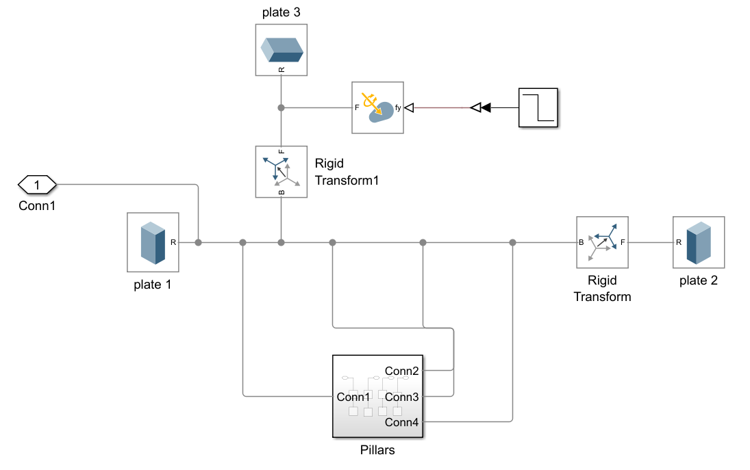
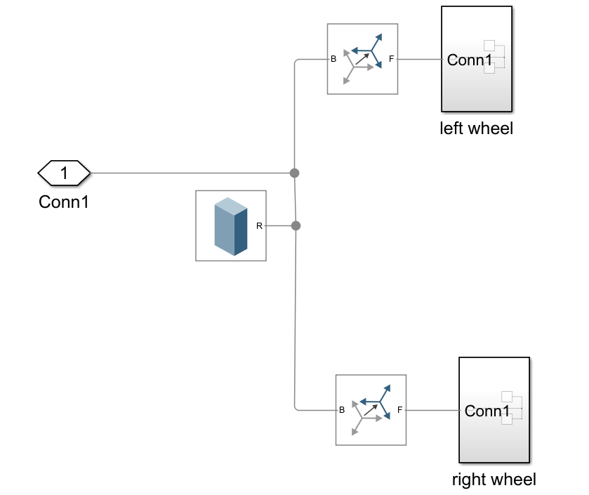
\[J\ddot{\theta}(t) \approx mgl\theta(t) + u(t)\]

I was able to provide first and define the world parameters and building of the robot via simscape library towards the simulation. I defined rigit transformations to connect initial cylindrical and rectangular blocks that was copied from a real-life robot toy. Furthermore, joints of revolute and prismatic was also defined towards how these will interact to each other with initial movement defined in terms of degree oscillations marked to be done for 10 seconds. The cart and the overall robot body simscape modelling is seen below.

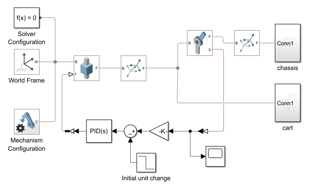
chassis body that models the robot body like the rods and plates above the wheels that needs balancing

cart body that models the shaft and the wheels of the robot

The input for the PID will be coming from the revolute joint angular velocity (denoted by q in the main simulink). The signal will be amplified further via a unit gain marked as \(-180/3.14\). This is via finding the radians which is just degrees/pi and has a negative value because gravity, our main force, is in the negative X-axis. This can be seen in the figure below. Inital unit step to decrease is set as 0 degrees with a step initial value to be 10 degrees and it lowers by 0.01 increments.

main simulink that provides the joints and how the PID interacts to the input from the revolute and tries to correct it to the prismatic joint.

2. PID Controller Equation

The PID control law is defined as:

\[u(t) = K_p e(t) + K_i \int_0^t e(\tau)\,d\tau + K_d \frac{de(t)}{dt}\]

Where:

( K_p ) = proportional gain
( K_i ) = integral gain
( K_d ) = derivative gain

In discrete form (as implemented in Simulink):

\[u[k] = K_p e[k] + K_i \sum_{i=0}^k e[i]\Delta t + K_d \frac{e[k] - e[k-1]}{\Delta t}\]

3. Control Loop Implementation

Sensor (or simulated block) measures tilt angle ( \theta(t) ).
Error ( e(t) ) is computed against the reference (0°).
PID computes control signal ( u(t) ).
Motors generate torque to counteract the tilt.
System repeats at each simulation step.

The tuned steady-response based on the scope block from simulink model. This is the block response in the comparison below.

Detailed PID parameters achieved for the self-balancing robot

Findings

Parameter Change	Observed Effect
↑ ( K_p )	Faster correction but may cause oscillations.
↑ ( K_i )	Eliminates steady-state error but can cause integral wind-up.
↑ ( K_d )	Provides damping, reduces overshoot and oscillation.
Output Saturation	Prevents unrealistic motor torque and avoids instability.

Before PID control tuning done that I have manually configured

After PID control tuning by the simulink PID Tuner App

Step Response Analysis

Settling time decreases as ( K_p ) increases.
Overshoot decreases as ( K_d ) increases.
Steady-state error approaches 0 with sufficient ( K_i ).

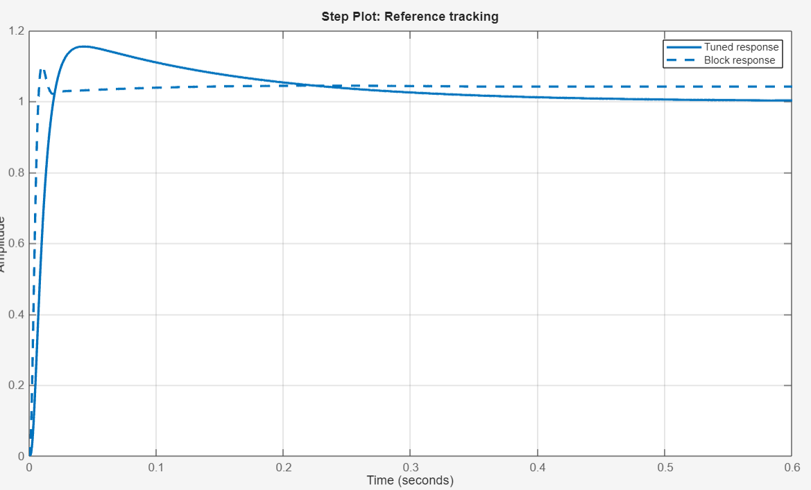
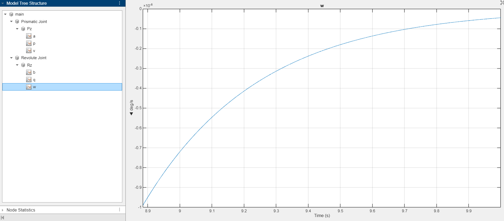
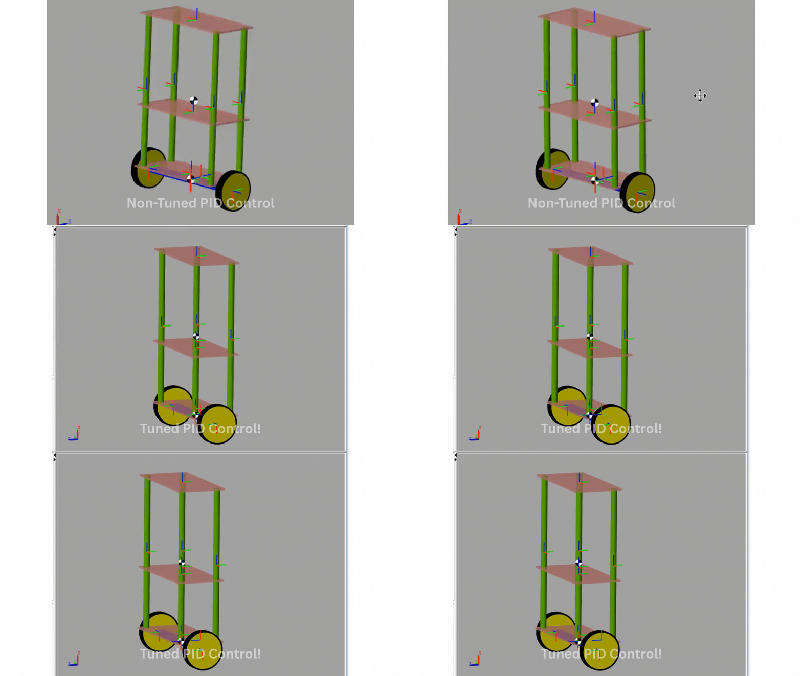
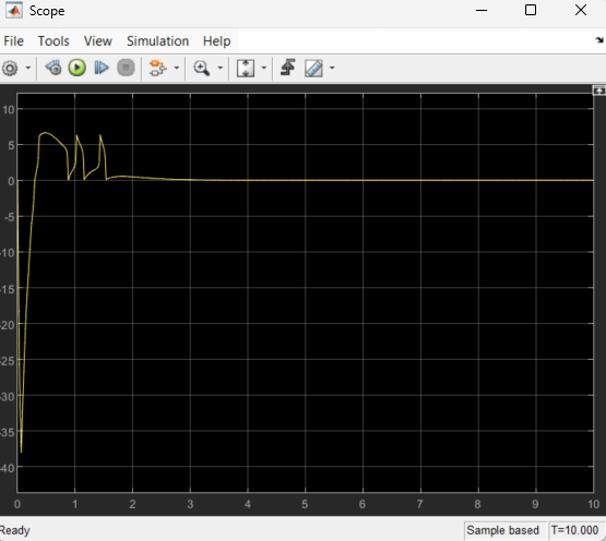
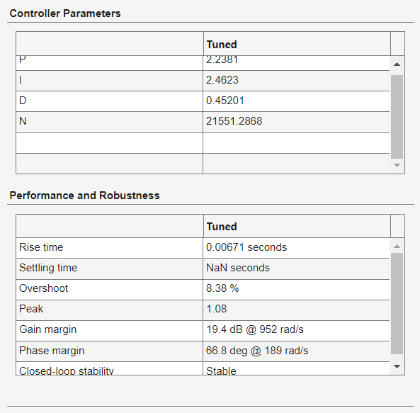
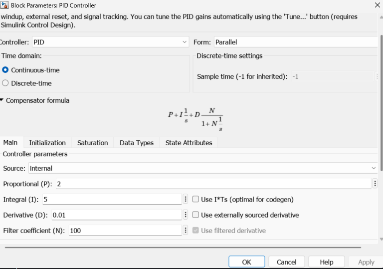
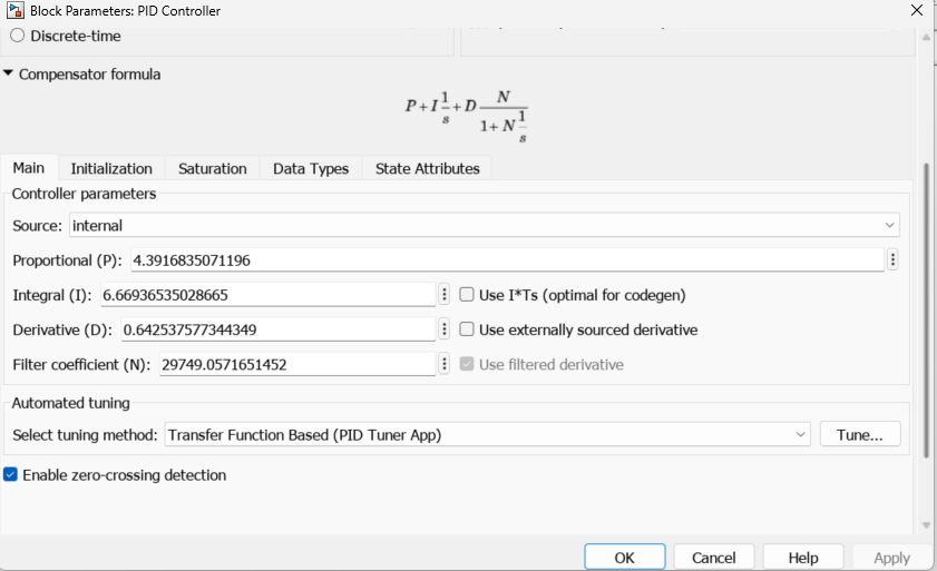
An indicator that the PID is working is by checking the tune response to the actual behavior. In this graph, we can see that the tuned response is remarkably close to the block response (the actual response) with an immediate flat value at the beginning.

data inspector that checks the angular velocity of the revolute joint. As you can see, PID control is as expected where angular velocity decrease over time which is our intended behavior!

As final comparison of the non-tuned PID control that I have manually made to the tuned control, below is a before and after the tuning. Sadly, I wanted to get its transfer function to define in mathematical representation the relationship of the I/O of the control system (idkh in the getting it in simulink control toolbox :<)

Before and after of the PID control after it was tuned. The oscillations brought by intiial pertubations have been significantly decreased where notable change in the filter coefficient and proportional were done to achieve this type of movement.

LEARNINGS:

Of course, this is not new, I have replicated this mostly from this github repository and youtube content which are excellent references that made this personal take about self-balancing robots possible with my own PID parameters that was eventually tuned for a steady-state response. This is an attempt to replicate their work and as addition to my learnings on how PID works in this simulation!

Suprisingly, the thing that I had the hard time to grasp was the simscape modelling as navigating the needed offsets for chassis definition under different coordinate system was a shot to the foot. So pro-tip is to define proper orientation and axes before modelling and eventual simulation!! The world configuration matters a lot.

Lastly, I have noticed that integral part of the was significantly under-utilized in the controller maybe due to the unit step error gradually decrease in the sum junction that lowers the needed corrective action to reduce the error when in fact the signal is already decreasing so more on the proportional-derivative action was needed to mitigate/correct error magnitude and know the rate of change from error. so maybe PD controller is better for this instance but I know for a fact that programmed sporadic pertubations will ensure that integral action will be needed as this is more needed in unpredictable environments.

I have also made a blog post relating to control systems. You may check it here particularly the learnings that I have made to define transfer functions and use of laplace transforms to solve differential equations.

HOW THIS PROJECT CAN BE FURTHER IMPROVED: The implementation that I did above consider an Angle PID where I was able to demonstrate how the control systems reduces the degree of the revolute joint in the wheels to about 1 degree of change. What would be cool is to also control the Speed with another PID to regulate further the robot's motion and movement. Another thing to look at is adding an LQR which stands for linear quadratic regulator is highly suggested as it improves on the immediate time response on the robots dyanamics and angle trajectory denote on the differential equation I have provided above. This would mean that instead of the robot wobbling, it will immediate reach a zero degree movement!